Negronis all round: simulation recovery of a discrete model 🍹
David Hodgson
2026-01-14
Example2.RmdThis vignette demonstrates how to recover a discrete latent variable model using simulated data on daily weather conditions and associated Negroni sales. The weather per day is a latent variable () that can take one of three states:
- Sunny ☀️,
- Cloudy ☁️
- Rainy 💧
and each state has its own distribution of Negroni sales 🍹. We’ll show how to infer the weather state for each day based on observed Negroni sales using a probabilistic modeling framework.
2. Simulated data
We simulate the dataset as follows:
Each day of a month has an unobserved (“latent”) weather state ($W_i ${🌧️, ☁️, ☀️ }). We assume each weather is equally likely to happen on each day. For each weather condition, we have a different distribution of Negroni sales each day which we assume follows:
- Sunny ☀️:
- Cloudy ☁️:
- Rainy 💧:
Based on this,let’s simulate some data:
set.seed(42)

# Parameters
n_days <- 30
weather_states <- c("sunny", "cloudy", "rainy")
lambda <- c(20, 10, 4)  # Poisson means for each weather state
prior_probs <- c(0.33, 0.33, 0.33)  # Prior probabilities for each weather state

# Generate latent weather states
latent_weather <- sample(weather_states, size = n_days, replace = TRUE, prob = prior_probs)

# Generate observed Negroni sales
sales <- sapply(latent_weather, function(w) {
  rpois(1, lambda[which(weather_states == w)])
})

# Combine into a data frame
data <- data.frame(day = 1:n_days, sales = sales, weather = latent_weather)

library(ggplot2)

# plot!
data %>%
  ggplot() +
    geom_col(aes(x = day, y = sales, fill = weather)) +
    scale_fill_manual(values = c("sunny" = "#f6cb2e", "cloudy" = "gray30", "rainy" = "#1eaefe")) +
    labs(x = "Day", y = "Negroni sales", fill = "Weather") + theme_bw()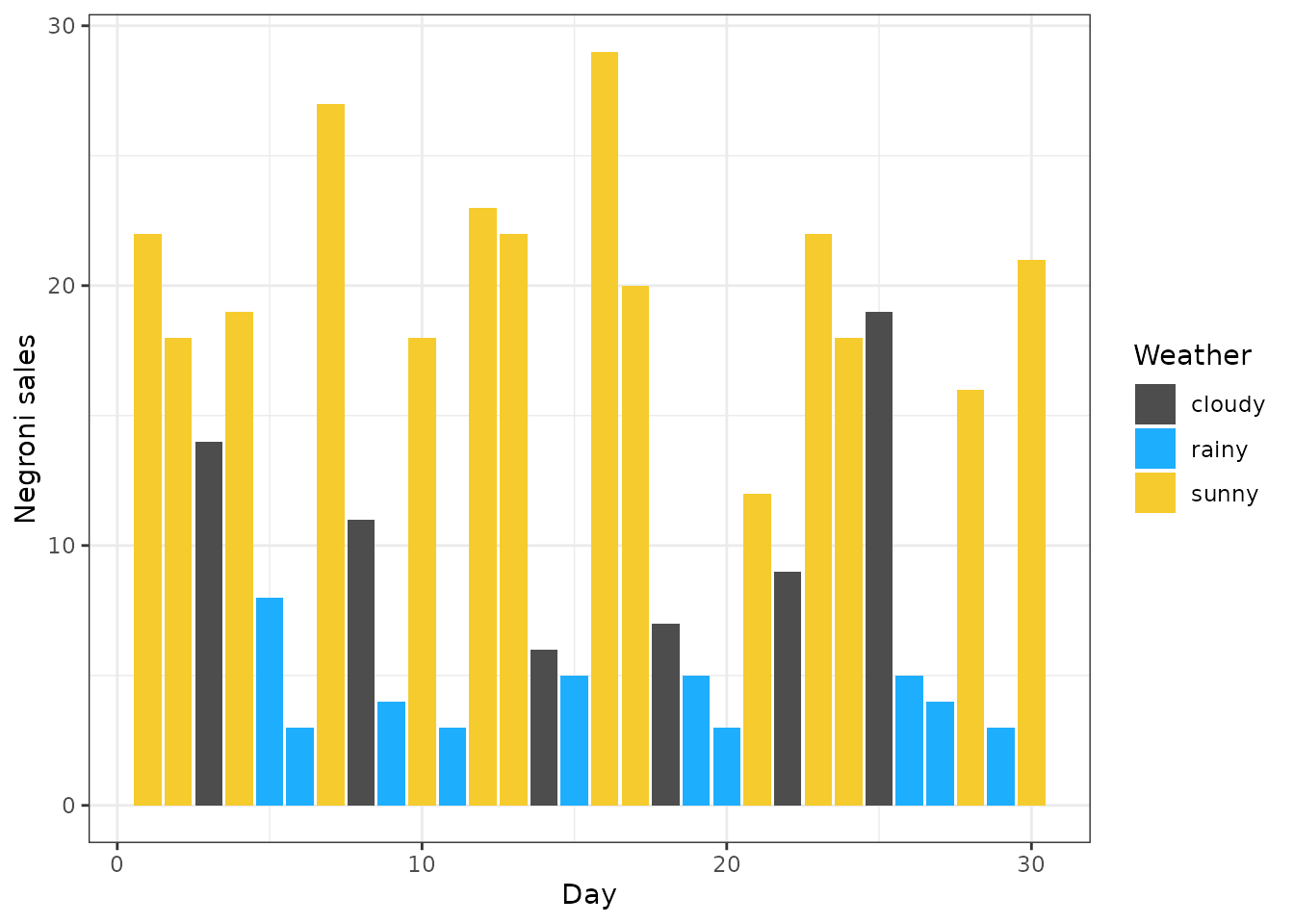
3. Simulation recovery
3.1 Description of the model
In our Bayesian model we assume that Observed Negroi Sales () are Poisson distributed with a rate parameter that depends on the latent weather state . That is the likelihood is Poisson with rate for each weather state . We assume the priors on the rate parameters . Finally, the prior distribution posterior distribution is given as the product of the likelihood and prior for each weather state .
3.2 Steps to Recover :
To recover the latent weather states, we use a Bayesian model with the following components:
Define the Likelihood Function: Implement the Poisson likelihood for given for each weather state .
Calculate the posterior probabilities: Use the likelihood and prior to compute the posterior probabilities for each using Bayes’ Rule.
Infer the model probable state per day: Assign each day to the weather state w with the highest posterior probability.
Repeat for all days: Perform the above inference for all days in the dataset to recover the sequence of latent weather states.
data_t <- list(
  N = nrow(data),
  y = data$sale
)

# Add all of these entries into a model list

model <- list(

# 1. Parameter Bounds (lowerParSupport_fitted and upperParSupport_fitted)
# These define the lower and upper bounds for the three model parameters: w_r, w_c, and w_s.
# w_r, w_c, and w_s are restricted to lie between 0 and 100.
# This ensures that the values for each parameter remain within a reasonable range during model fitting or sampling.

  lowerParSupport_fitted = c(0, 0, 0),
  upperParSupport_fitted = c(100, 100, 100),

# 2. Parameter Names (namesOfParameters)
# namesOfParameters is a vector containing the names of the three parameters that the model will estimate:
#w_r: the rate associated with the first category (discrete value 1),
#w_c: the rate associated with the second category (discrete value 2),
#w_s: the rate associated with the third category (discrete value 3).
  namesOfParameters = c("w_r", "w_c", "w_s"),

## 3. Discrete Length (discrete_length)
# This is the length of the discrete sequence (i.e., the number of data points N). The model assumes that discrete has a length of 30, meaning there are 30 discrete latent variables to be inferred from the data, corresponding to 30 days.
  discrete_length = 30,

# 4. Sampling from Prior Distributions (samplePriorDistributions)
## The function samplePriorDistributions generates prior samples for the parameters w_r, w_c, and w_s.
## It samples each parameter independently from a uniform distribution between 0 and 100.

  samplePriorDistributions = function(datalist) {
    runif(3, 0, 100)
  },

# 5. Evaluating the Log-Prior (evaluateLogPrior)
# The function evaluateLogPrior calculates the log-prior of the model based on the parameters params (a vector containing w_r, w_c, and w_s).
  evaluateLogPrior = function(params, discrete, datalist) {

    lpr <- dunif( params, 0, 100, TRUE) %>% sum
    if (!(params[1] < params[2] & params[2] < params[3])) {
      lpr <- log(0)
    }
    lpr
  },

# 6. Initialising the Discrete Latent Variables (initialiseDiscrete)
# initialiseDiscrete initializes the discrete latent variables for each data point.
# The function samples N values (where N = 30 in this case) from the set {1, 2, 3}, assigning each data point to one of the three possible categories. This is done randomly with replacement.
  initialiseDiscrete = function(datalist) {
      require(purrr)

      N <- datalist$N

      discrete <- sample(1:3, N, replace = TRUE)
      discrete
    },

#7. Discrete Sampling (discreteSampling)
# discreteSampling is a function that updates the latent discrete variable using a random walk approach. It applies a random operation (based on the value of u) to the current state of the discrete vector:
#With probability 1/3, it randomly resamples one element of the discrete vector and assigns it to a new value from the set {1, 2, 3}.
#With probability 1/3, it swaps the values of two randomly selected elements in the discrete vector.
#With the remaining probability, no change is made to the discrete vector.
    discreteSampling = function(discrete, datalist) {

        u <- runif(1)
        N <- datalist$N
        # resample
        if (u < 0.33) {
          j <- sample(1:N, 1)
          discrete[j] <- sample(1:3, 1)
          # swap
        } else if(u < 0.66) {
          j_idx <- sample(1:N, 2)
          j_idx_1 <- discrete[j_idx[1]]
          discrete[j_idx[1]]  <- discrete[j_idx[2]]
          discrete[j_idx[2]] <- j_idx_1
        } else {
          # nothing happens!
        }
        return(discrete)
    },

# 8. Evaluating the Log-Likelihood (evaluateLogLikelihood)
# The function evaluateLogLikelihood calculates the log-likelihood for a set of parameter values params, given the observed data and the current state of the discrete latent variables.
# w_r, w_c, and w_s are the three model parameters (rates).
# The function iterates over each data point (from 1 to N, where N = 30), checking which category (discrete[i]) the data point belongs to.
#For each category (1, 2, or 3), it calculates the log-likelihood of the observed data point datalist$y[i] under the corresponding Poisson distribution with the rate parameter (w_r, w_c, or w_s).
#The log-likelihood is accumulated and returned as the total log-likelihood for the model.
  evaluateLogLikelihood = function(params, discrete, covariance, datalist) {
    w_r <- params[1]
    w_c <- params[2]
    w_s <- params[3]

    N <- datalist$N
    ll <- 0;
    for (i in 1:N) {
      if (discrete[i] == 1) {
         ll <- ll + dpois(datalist$y[i], w_r, log = TRUE)
      } else if (discrete[i] == 2) {
         ll <- ll + dpois(datalist$y[i], w_c, log = TRUE)
      } else {
         ll <- ll + dpois(datalist$y[i], w_s, log = TRUE)
      }

    }
    ll
  }
)
3.3. Settings and run model
Select the run time, chains, number of cores, burnin and thinning for the model.
# Settings used for the ptmc model
settings <-  list(
  numberChainRuns = 2,
  numberCores = mc.cores,
  numberTempChains = 10,
  iterations = 100000,
  burninPosterior = 50000,
  thin = 100
)

post <- ptmc_discrete_func(model=model, data=data_t, settings=settings)
4. Analyse the posterior distributions
ptmc_discrete_func returns a list of with entries:
- : An MCMC object with posterior samples of the model parameters.
- : A list of discrete states generated during the simulation for each chain.
- : A data frame of log-posterior values, with columns representing different chains and rows representing samples.
- : A data frame of temperatures for each chain at each sample.
- : A data frame of acceptance rates for each chain at each sample.
- : A list containing the parameter values for each chain.
. The first entry is post$mcmc a mcmc or mcmc.list
object (from the coda package). You can plot these and
calculate convergence diagnostics using coda functions:
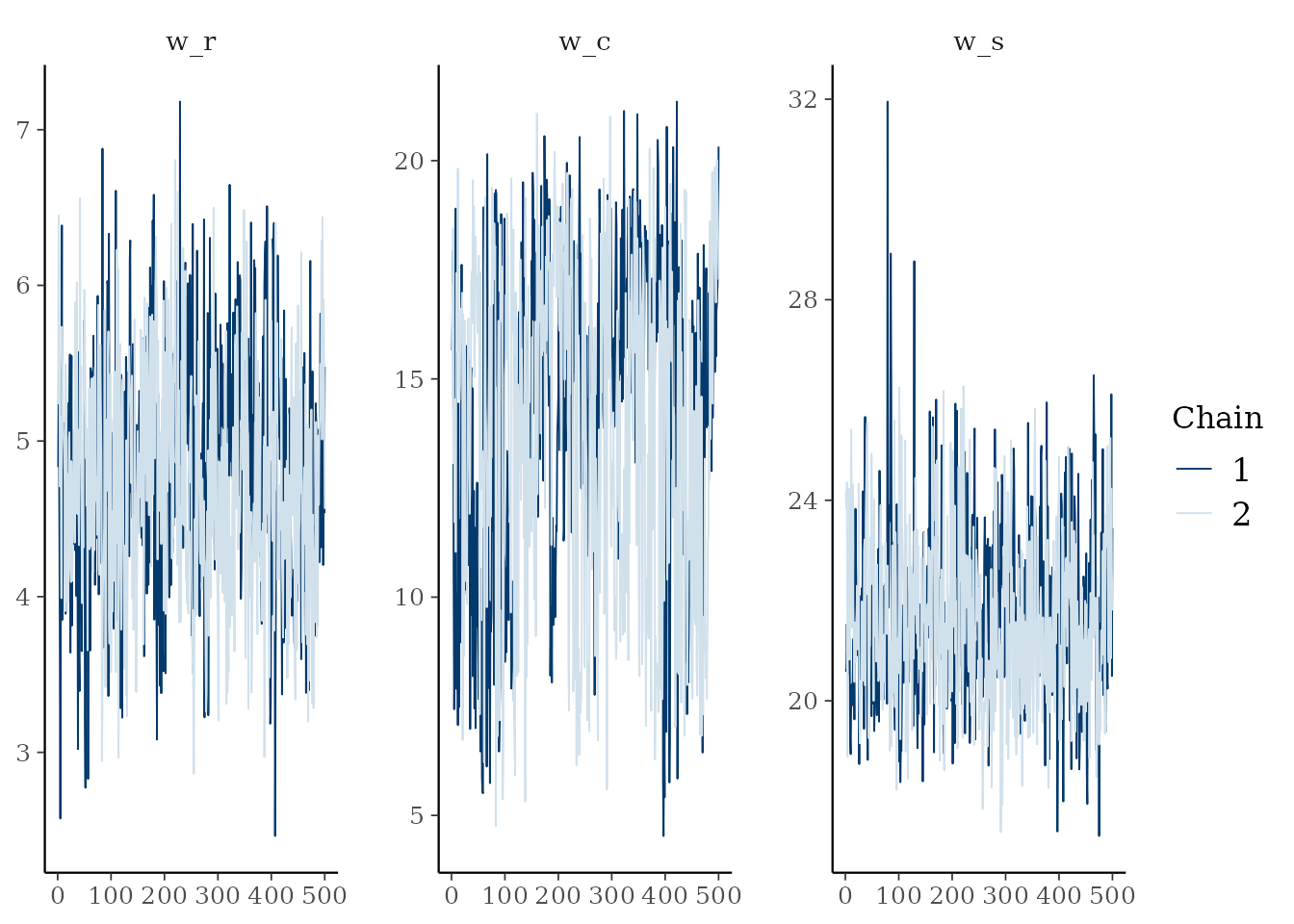
# Plot the Gelman-Rubin diagnostic for the parameters
gelman.plot(post$mcmc)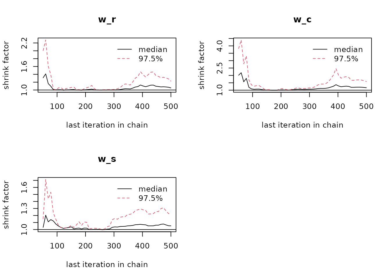
The next entry is post$lpost and is long table dataframe
of the log-posterior values. These values can be easily plotted using
ggplot2:
library(ggplot2)


# Plot of the logposterior for the three chains
lpost_conv <- post$lpost %>% filter(sample_no>250)
logpostplot <- ggplot(lpost_conv, aes(x = sample_no, y = lpost)) +
  geom_line(aes(color = chain_no), size = 0.2, alpha=0.8) +
  theme_minimal()
logpostplot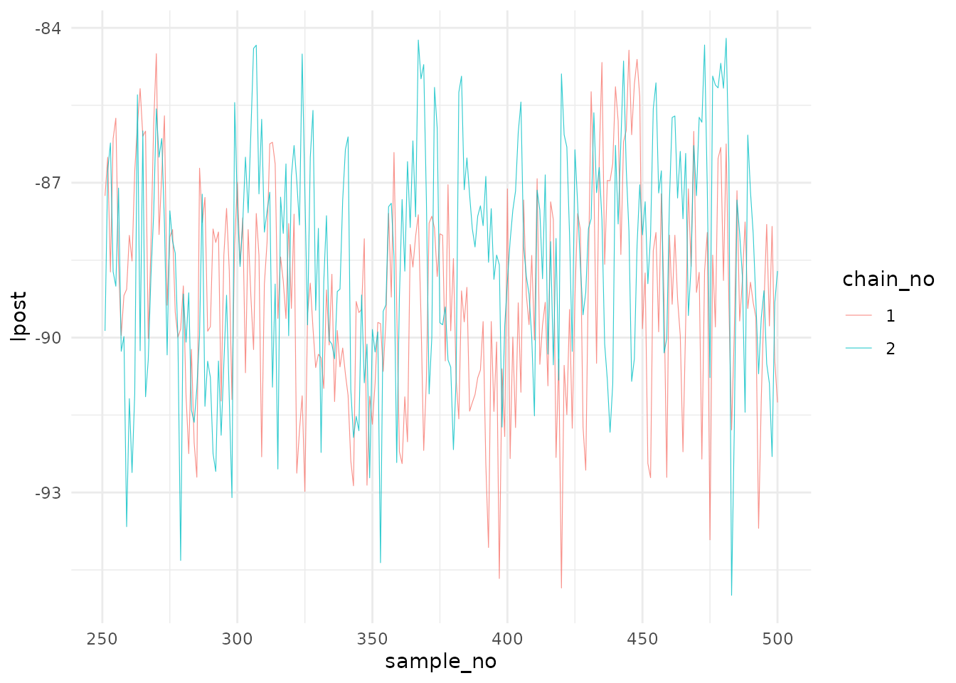
The next entry is post$discrete and is a list of
matrices describing the discrete states for each chain. These can be
easily plotted using ggplot2 also:
library(purrr)
df_discrete <- make_long_discrete(post$discrete)

weather_key <- c("1" = "rainy", "2" = "cloudy", "3" = "sunny")

df_discrete_plt <- df_discrete %>% mutate(value = recode(value, !!!weather_key)) %>%
    mutate(idx = factor(idx, levels = 1:30))

 df_discrete_plt   %>%
  ggplot() +
    geom_col(aes(x = idx, y = sample_no, fill = factor(value))) +
    scale_fill_manual(values = c("sunny" = "#f6cb2e", "cloudy" = "gray30", "rainy" = "#1eaefe")) +
    theme_minimal() + labs(x = "Sample number", y = "Weather state", fill = "Weather")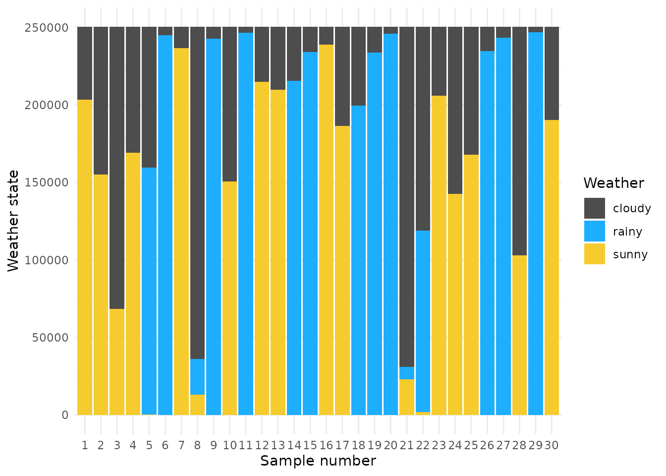
Let’s find the most probable weather state for each day based on the posterior samples and compare it to the true weather state (box color below 0.0)
recode_emoji <- c("sunny" = "\U1F602", "cloudy" = "☁️", "rainy" = "🌧️")
recode_emoji_color <- c("sunny" = "#f6cb2e", "cloudy" = "gray30", "rainy" = "#1eaefe")

true_sim <- data.frame(
    idx = 1:30,
    true = latent_weather
) %>% mutate(color = recode(true, !!!recode_emoji_color)) %>%
  mutate(true_emoji = recode(true, !!!recode_emoji))


S <- df_discrete_plt$sample_no %>% unique %>% length

df_discrete_plt_mode <- df_discrete_plt %>% group_by(idx, value) %>%
    summarise(n = n() / S) %>% filter(n == max(n))
df_discrete_plt_mode %>%
    ggplot() +
      geom_col(aes(x = idx, y = n, fill = factor(value))) +
      geom_rect(data = true_sim, aes(xmin = idx - 0.3, xmax = idx + 0.3, ymin = -0.3, ymax = -0.1, fill = true)) +
      scale_fill_manual(values = c("sunny" = "#f6cb2e", "cloudy" = "gray30", "rainy" = "#1eaefe")) +
      theme_minimal() + labs(x = "Sample number", y = "Weather state", fill = "Weather")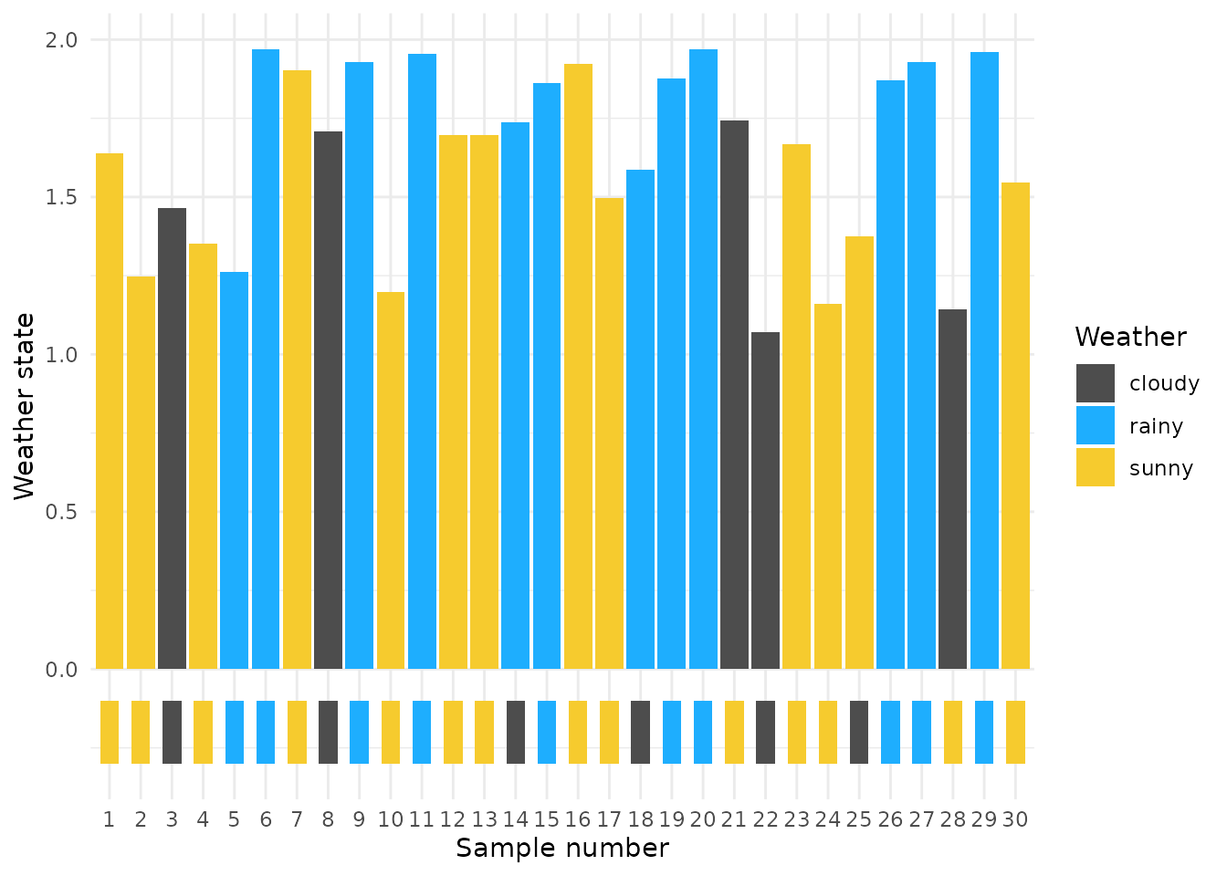
## 5. simulation recovery metrics
Here are a few easy distance metrics to compare the true and recovered weather states.
5.1. Simple Matching Coefficient (SMC)
The SMC calculates the proportion otrue_sim f elements in the vectors that match exactly.
recode_number <- c("sunny" = "3", "cloudy" = "2", "rainy" = "1")


true_vec <- true_sim %>% mutate(true_num = recode(true, !!!recode_number)) %>% pull(true_num)
model_est_vec <- df_discrete_plt_mode %>% mutate(value_num = recode(value, !!!recode_number)) %>% pull(value_num)


# SMC calculation
smc <- sum(true_vec == model_est_vec) / length(true_vec)
smc
## [1] 0.8