Continuous only model

David Hodgson

2024-11-21

#devtools::install("..") #install if needed
library(ptmc)
library(dplyr)
library(tidyr) 
library(coda)


# Using more than one core might fail on windows, 
if (.Platform$OS.type == "windows") {
  mc.cores <- 1
} else {
  mc.cores <- 2 # use as many as available, preferably 4.
}

Parallel Tempering Monte Carlo

Model

The example model is taken from Ben Lambert’s fantastic book, “A Student’s Guide to Bayesian Statistics,” Questions 13.3. Briefly, I assume the random count variable $X_t$, the number of mosquitos caught during day $t$, is Poisson, such that

$$\begin{split} X_t &\sim \textit{Poisson}(\lambda)\\ \lambda &= 1000 \times \exp(-\mu t)\psi \end{split}$$

where $\mu$ is a constant mortality hazard rate and $\psi$ is the daily recapture probability with prior distributions of $\mu \sim \Gamma(2,20)$ and $\psi \sim \textit{Beta}(2, 40)$. The data $x_t$, the number of mosquitos caught on day $t$, are given in the RWM_mosquito.csv file but can also be found here.

Implementation

Create the model

The model list should be a list with three functions, samplePriorDistributions, evaluateLogLikelihood, and evaluateLogPrior and a vector string with the parameter names used in the calibration, namesOfParameters.

vector string par_names

A vector string of the parameter names.

func samplePriorDistributions

A function which generates the initial values (usually by sampling the prior distributions)

• (no arguments)
• @return vector of values

func evaluateLogLikelihood

A function which generates the log-likelihood for a set of parameter values

• @param data, data needed to calculate the log-likelihood
• @param params, parameter values
• @return log-likelihood

func evaluateLogPrior

A function which calculates the log-prior for a set of parameter values

• @param params, parameter values
• @return log-prior

# model is a list of three functions and a vector string
model <- list(

  lowerParSupport_fitted = c(0, 0),
  upperParSupport_fitted = c(10, 1),


  namesOfParameters = c("mu","psi"),

  samplePriorDistributions = function(datalist) {
    c(rgamma(1, 2, 20), rbeta(1, 2, 40))
  },

  evaluateLogPrior = function(params, datalist) {
    if (params[1] < 0 || params[2] < 0 || params[1] > 1 || params[2] > 1)
      return(-Inf)

    lpr <- 0
    lpr <- lpr + log(pgamma( params[1], 2,20))
    lpr <- lpr + log(pbeta( params[2], 2,40))
    lpr
  },

  evaluateLogLikelihood = function(params, covariance, datalist) {
    y <- datalist$y
    mu <- params[1]
    psi <- params[2]
    ll <- 0;
    for (t in 1:length(datalist$y))
    {
      sum_x = 0
      lambda = 1000*exp(-mu*(t+1))*psi;
      for (i in 1:y[t]){
        sum_x <- sum_x + i
      }
      ll <- ll - lambda + y[t]*log(lambda) - sum_x
    }
    ll
  }
)

Obtain the data

Data used in the log-likelihood function can be in any format.

dataMos <- read.csv("RWM_mosquito.csv") 
# restructure the data for the log-likelihood function
data_t <- list(
  time = dataMos$time,
  y = dataMos$recaptured
)

data_t

## $time
##  [1]  1  2  3  4  5  6  7  8  9 10 11 12 13 14 15
## 
## $y
##  [1] 39 21 36 34 18 22 43 11 17  9 15 11 13 13  7

Settings

The settings for the parallel tempering algorithm are summarised here.

Settings Options

• numberChainRuns, number of independent chains to run
• numberTempChains, number of dependent chains per chain run (i.e. the number of rungs in the temperature ladder)
• iterations, the number of steps to take in the Markov chain, (including the burn-in)
• burninPosterior, the number of steps in the burn-in (these are discarded)
• thin, thinning of the chain (i.e. =10 means only every 10th sample is saved)
• consoleUpdates, frequency at which the console updates (i. =100 means every 100th step)
• numberFittedPar, number of parameters
• onAdaptiveCov, whether to include adaptive covariance
• updatesAdaptiveCov, frequency at which the adaptive covariance matrix is updated
• burninAdaptiveCov, number of steps to take before using the adaptive covariance matrix
• onAdaptiveTemp, whether to include adaptive temperature ladder
• updatesAdaptiveTemp, frequency at which the adaptive temperature ladder is updated
• Debug, run with debug output

# settings used for the ptmc model 
settings <-  list(
  numberChainRuns = 2,
  numberTempChains = 10,
  iterations = 10000,
  burninPosterior = 5000,
  thin = 10,
  consoleUpdates = 100,
  numberFittedPar = 2,
  onAdaptiveCov = TRUE,
  updatesAdaptiveCov = 200,
  burninAdaptiveCov = 100,
  onAdaptiveTemp = TRUE,
  updatesAdaptiveTemp = 10,
  onDebug = FALSE,
  lowerParBounds = model$lowerParSupport_fitted,
  upperParBounds = model$upperParSupport_fitted,
  covarInitVal = 1e-8, # make very small if struggling to sample to beginning
  covarInitValAdapt = 1e-4, # make very small if struggling to sample to beginning
  covarMaxVal = 1, # decrease if struggling to sample in the middle
  runParallel = TRUE,
  numberCores = mc.cores
)

Run the model.

post <- ptmc_func(model=model, data=data_t, settings=settings)

Plot the data

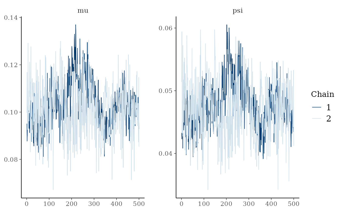
ptmc_func returns a list of length two. The first entry is post$mcmc a mcmc or mcmc.list object (from the coda package). I can plot these and calculate convergence diagnostics using coda functions:

library(posterior)
library(coda)
library(bayesplot)
summary(post$mcmc)

post$mcmc %>% mcmc_trace

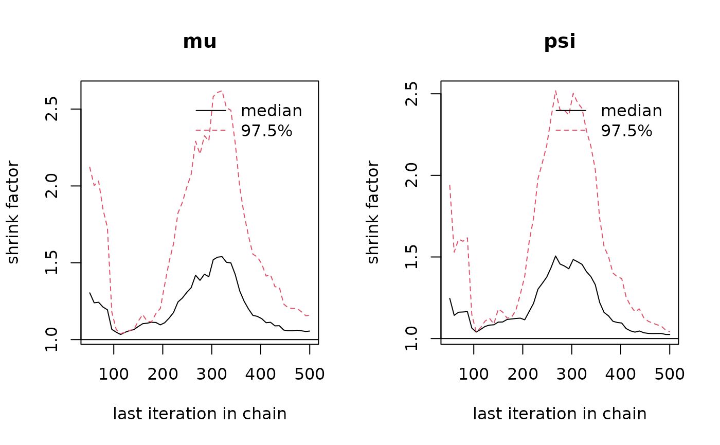
# Plot the Gelman-Rubin diagnostic for the parameters
gelman.plot(post$mcmc)

gelman.diag(post$mcmc)

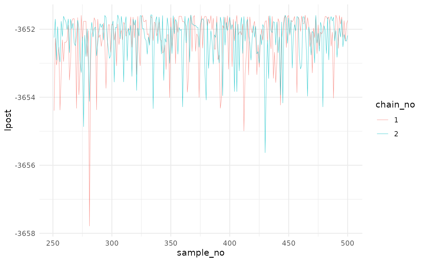
The second entry is post$lpost and is long table dataframe of the log-posterior values. These values can be easily plotted using ggplot2:

library(ggplot2)

# Plot of the logposterior for the three chains
lpost_conv <- post$lpost %>% filter(sample_no>250)
logpostplot <- ggplot(lpost_conv, aes(x = sample_no, y = lpost)) + 
  geom_line(aes(color = chain_no), size = 0.2, alpha=0.8) +
  theme_minimal()

## Warning: Using `size` aesthetic for lines was deprecated in ggplot2 3.4.0.
## ℹ Please use `linewidth` instead.
## This warning is displayed once every 8 hours.
## Call `lifecycle::last_lifecycle_warnings()` to see where this warning was
## generated.

logpostplot

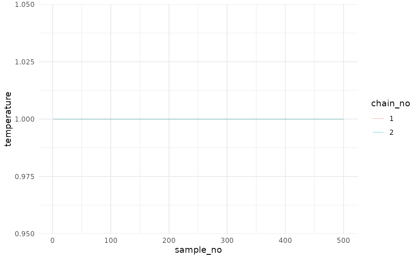
The third entry is post$temp and is long table dataframe of the adaptive temperature values. These values can be easily plotted using ggplot2:

tempplot <- ggplot(post$temp, aes(x = sample_no, y = temperature)) + 
  geom_line(aes(color = chain_no), size = 0.2, alpha=0.8) +
  theme_minimal()

tempplot